/home/andrew$

17 papers, 2.6 sigmas, and 1 event

The LZ experiment recently announced (1 September) a new result through a talk and preprint paper.

The paper documents something strange: a single, unexplained event that could be consistent with an interaction with a Dark Matter particle. The data were analysed using frequentist, and specifically Fisherian, statistical methods described here. In particular, evidence was quantified using a \(p\)-value, that is, the probability of obtaining data that were at least as extreme as that observed given the background-only (i.e., no Dark Matter) hypothesis. The \(p\)-value was about 0.5%. For historical reasons, this is communicated as \(2.6\sigma\), as 0.5% corresponds to the probability mass contained in the tail of a Normal distribution at \(Z = 2.6\).

Hey ho, you might think. That ain't much evidence for an extraordinary claim, especially since it is contingent on their background and detector modeling to the 1 rogue-event level, and given all we know about \(p\)-values, the replication crisis, and the strength of evidence. That said, it might just about be below a threshold proposed by Benjamin et al. (2017) in social and medical sciences, thought not close to the physics typical requirement of \(5\sigma\) for a discovery.

In the two days that followed the paper, however, there were 17 theory papers that presented particular models of Dark Matter that could explain that 1 event. Hmm. I haven't read them well enough to comment on how well-motivated these explanations are, though the most popular appears to be a Higgsino explanation (see e.g., Fan & Reece), where a supersymmetric partner of the Higgs plays the role of Dark Matter. However, a paper today suggests Higgsinos may be in tension with so-called sideband results from LZ. That means, they would predict Dark Matter signals in other searches performed by LZ, but none were seen.

There was a particular statement in Fan & Reece that caught my eye:

The look-elsewhere correction depends on the total number of models that were fit to the data, and as such is arguably too conservative when, as we will argue, there is one particularly compelling model to focus on

Hmm. One of the infamous things about \(p\)-values is that they depend on the experimentalists' analysis plan. That is, they depend on what the experimentalists would have done, were the data different. Part of computing them correctly thus involves correcting for the look-elsewhere effect (LEE). This means, correcting for all the things you, the experimenter, would have looked at had the data been different. There is a famous reductio ad absurdum about a statistician and electrician, by Edwards and Pratt, described here that shows how strange this can be.

The long-and-short of this is that the \(p\)-value depends on the experimentalists' analysis plan, which should ideally be declared before data collection. I don't think it's reasonable to claim after the fact that

Ah! But I was only interested in this subset of tests anyway (which happened to include tests that produce the smallest \(p\)-values). Let's just use those ones. Thus the \(p\)-value is smaller!

This would have been perfectly fine pre-data. I would have no objection to pre-data, or pre-unblinding of data, someone saying, let's use an analysis plan that only performs these tests to maximise the statistical power for these particular Dark Matter models that we find plausible. Post-data, however, it's too late, at least within a frequentist paradigm.

On the other hand, perhaps Fan & Reece are subconsciously thinking as Bayesians. In Bayesian frameworks, we don't need to consider the sampling plan or what we'd have done were the data different: our conclusions depend only on the data we did observe. This is connected to the likelihood principle. In that case, perhaps a more charitable interpretation is that:

Ah! I don't care about your error rates and what you'd have done were data different. I just care about what I should believe given the data at hand. The Dark Matter models that explain the event were a priori plausible to me. Given that, I am more inclined to believe that they explain the data.

I think that's a defensible point of view.

Tags: dark-matter, statistics, physics

Curious trends in arXiv submission data

There was a curious discussion at Peter Woit's blog concerning recent arXiv submission trends. It was observed (after some initial confusion) that the number of revisions appeared to have increased dramatically in the last month or so.

An (AI generated) analysis, available on GitHub, confirmed this pattern. The data look like this.

What causes that surge in revisions (red) versus posts (blue)? This recent trend appears in all arXiv categories. The AI declares that it is a real trend and speculates that authors are submitting revisions using generative AI tools. I'm naturally skeptical, so thought someone should least build a statistical model of what this plot might look like, assuming nothing but a stationary process.

So I did. I took submissions per month to be about 250 $$ n \sim \textrm{Po}(250) $$ and assumed that authors posted a revision upon publication to match the published version, about six months later, $$ d \sim \textrm{Po}(6) $$ What do you know?

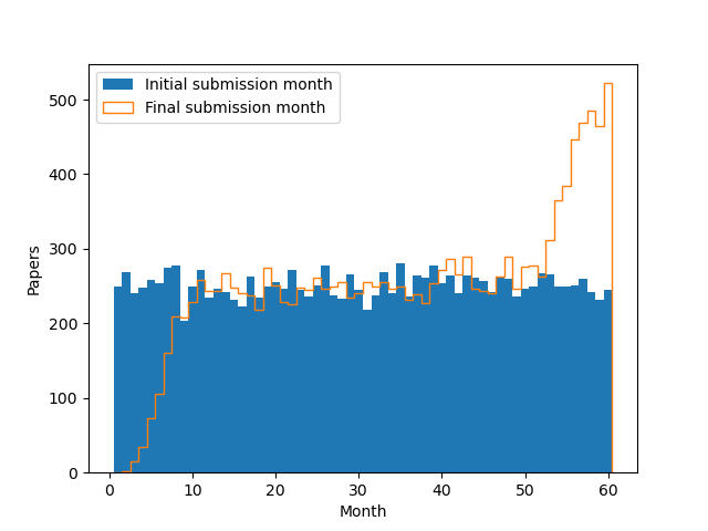
In the current month (here month 60), you see the first submissions (that haven't been replaced yet) and revisions (from papers from previous months). In past months, you only see revisions, as the first submissions are later replaced.

This was an interesting example of a stationary that process produces a mirage of non-stationary behaviour (a surge in the current month). The explanation about AI revisions is unwarranted. On the other hand, there is almost certainly non-stationary behavior in the dataset, as, e.g., the number of academics has increased over time.

Don't take my word for it, of course. Run it yourself. I'd love to see a Bayesian analysis that constructed a principled model and fitted it to the actual data.

"""
arXiv submission patterns
=========================
"""

import numpy as np
import matplotlib.pyplot as plt

rate_per_month = 250
publication_time_months = 6
end_month = 60  # 5 years


def simulate():

    # make papers
    initial = []
    for i in range(end_month):
        initial += np.random.poisson(rate_per_month) * [i + 1]

    # now post a new version after publication some time later
    published = [a + np.random.poisson(publication_time_months)
                 for a in initial]

    # final update before end of simulation
    final = [b if b <= end_month else a for a, b in zip(initial, published)]

    return initial, final


if __name__ == "__main__":

    initial, final = simulate()

    bins = np.arange(0.5, end_month + 1, 1)

    plt.hist(initial, bins=bins, label="Initial submission month")
    plt.hist(final, bins=bins, histtype="step", label="Final submission month")
    plt.legend()
    plt.xlabel("Month")
    plt.ylabel("Papers")
    plt.savefig("arxiv.png")

Tags: code, ai, arxiv, statistics